#30DayMapChallenge Day 5: Late Quaternary Precipitation in Southwest Asia

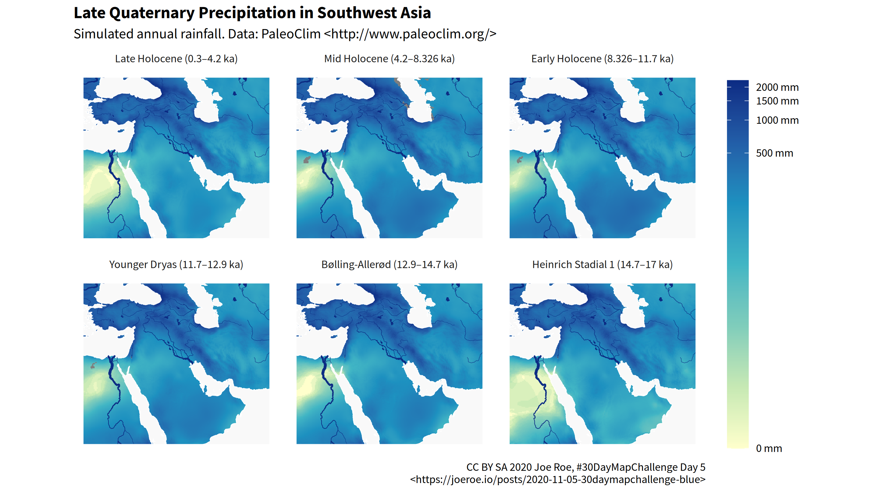
The theme for day 5 of the #30DayMapChallenge is “blue”. My submission is a map of simulated rainfall in Southwest Asia during key climate periods in the Late Quaternary.

The map was generated in R using the code below. View the RMarkdown source on GitHub.

library("tidyverse")
library("sf")
library("raster")
library("stars")
library("glue")
library("rnaturalearth")
library("ragg")

# remotes::install_github("joeroe/rpaleoclim")
library("rpaleoclim")

Data

I used reconstructed climate data from PaleoClim. My package rpaleoclim makes getting data from PaleoClim more straightforward.

sw_asia <- extent(c(25, 65, 15, 45))

tribble(
  ~code, ~name,                ~start, ~end,
  "lh",  "Late Holocene",      4.2,    0.3,
  "mh",  "Mid Holocene",       8.326,  4.2,
  "eh",  "Early Holocene",     11.7,   8.326,
  "yds", "Younger Dryas",      12.9,   11.7,
  "ba",  "Bølling-Allerød",    14.7,   12.9,
  "hs1", "Heinrich Stadial 1", 17.0,   14.7
) %>% 
  mutate(paleoclim = map(code, paleoclim, region = sw_asia)) %>% 
  mutate(paleoclim = map(paleoclim, subset, subset = "bio_12")) ->
  palclim

As always, Natural Earth provides the base layers.

ocean <- ne_download(scale = 10, type = "ocean", category = "physical",
                     returnclass = "sf")
lakes <- ne_download(scale = 10, type = "lakes", category = "physical",
                     returnclass = "sf")
rivers <- ne_download(scale = 10, type = "rivers_lake_centerlines_scale_rank", 
                      category = "physical", returnclass = "sf")

ocean <- st_make_valid(ocean)
ocean <- st_crop(ocean, sw_asia)
lakes <- st_crop(lakes, sw_asia)
rivers <- st_crop(rivers, sw_asia)

Plot

I converted the palaeoclimate data from Raster to stars format, since the latter makes it easier to combine raster and sf vector layers.

palclim$paleoclim %>% 
  stack() %>% 
  st_as_stars() %>% 
  st_set_dimensions("band", 
                    values = glue_data(palclim, "{name} ({end}–{start} ka)")) ->
  palclim_cube

ggplot() +
  geom_stars(data = palclim_cube) +
  geom_sf(data = ocean, fill = "#f9f9f9", colour = "#ffffff", size = 0.25) +
  geom_sf(data = rivers, mapping = aes(size = strokeweig / 2),
          colour = "#0c2c84") +
  geom_sf(data = lakes, fill = "#0c2c84", colour = NA) +
  geom_sf(data = sw_asia %>% as("SpatialPolygons") %>% st_as_sf() %>% st_set_crs(4326),
          fill = NA, colour = "#ffffff", size = 0.5) +
  scale_fill_distiller(palette = "YlGnBu", direction = 1, trans = "pseudo_log",
                       labels = function(x) paste(x, "mm"),
                       guide = guide_colourbar(title = NULL,
                                               frame.colour = "#ffffff",
                                               ticks.colour = "#ffffff",
                                               barheight = unit(0.75, "snpc"))) +
  scale_size_identity() +
  facet_wrap(~band) +
  labs(
    x = NULL, y = NULL, 
    title = "Late Quaternary Precipitation in Southwest Asia",
    subtitle = "Simulated annual rainfall. Data: PaleoClim <http://www.paleoclim.org/>",
    caption = paste("CC BY SA 2020 Joe Roe, #30DayMapChallenge Day 5",
                   "<https://joeroe.io/posts/2020-11-05-30daymapchallenge-blue>",
                   sep  = "\n")
  ) +
  theme_minimal(
    base_family = "Source Sans Pro",
  ) +
  theme(
    plot.title = element_text(face = "bold"),
    axis.text = element_blank(),
    panel.grid = element_blank(),
  )